SULFUR AND CARBON ISOTOPES ACROSS THE ARCHEAN AND PALEOPROTEROZOIC
|
In order to gain a better understanding of the geochemical changes that were occurring on the early Earth as it transitioned from a reducing to oxidizing atmosphere (aka the Great Oxidation Event, or GOE, that happened 2.45 billion years ago), we undertook compiling literature values for δ34S, Δ33S, and Δ36S from sulfide and sulfate minerals as well as δ13C for carbonate minerals and organic carbon. The result was approximately 20,000 data points compiled and a review paper in Earth Science Reviews (link to paper below). The data set we have made available as a excel spreadsheet so that the scientific community can benefit from having this data set freely available to plot and add to. This effort was done with the help of Dr. Aviv Bachan, Prof. Trinity Hamilton, and Dean Lee Kump while all of us were at Penn State.
We found that there appeared to be four distinct time periods as recorded in the S and C isotope data. We proposed these four steps to be 1) the Eoarchean through the Mesoarchean (4.00 to 2.80 Ga), 2) the Neoarchean (2.80 to 2.45 Ga), 3) the first part of the Paleoproterozoic (2.45 to 2.00 Ga), and then 4) the second part of the Paleoproterozoic and on into the Mesoproterozoic (after 2.00 Ga). We also suggested the Great Oxidation Event (which is the boundary between the Archean and Proterozoic) should be placed at ~2.45 Ga, and that the Paleoproterozoic be broken up into two eras: a new 'Eoproterozoic' (2.45 to 2.00 Ga) and a shortened Paleoproterozoic (2.00 to 1.60 Ga). We also folded in the onset and evolution of microbially mediated metabolic pathways and processes, focusing on those involved with the sulfur cycle and carbon cycle. Based on our observations, we then brought in some speculation on the timing of the onset of carbon and sulfur metabolisms based on the S and C isotope record to help with hypothesis generation in testing through geochemical proxies as well as molecular clock techniques. We are now using this data compilation to explore and interpret ancient systems as well as using modern systems as proxies to help explain values.
Below is a link to the paper, where you can also download the data set as an excel spreadsheet:
https://www.sciencedirect.com/science/article/pii/S0012825216304305
|
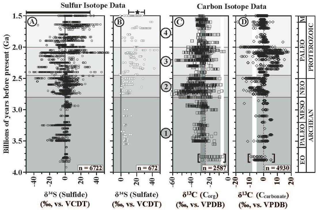
Figure 1 (above) from our review paper on sulfur and carbon isotope data from 4.0 to 1.5 Ga. This plot shows the trends in the data for δ34S in sulfide (A) and sulfate (B) minerals and δ13C data in organic carbon (C) and carbonate minerals (D). For associated literature sources for this and the following figures, please check out the paper. For sulfide and sulfate mineral S isotopic data, mantle values (~ 0 per mil) are shown, as well as bars showing the range of modern mineral values (star = ocean sulfate values of ~ 21 per mil). For organic carbon isotopic data the white bar shows mantle values, and the dashed line and grey bar show expected carbon fractionation due to biological carbon fixation. Carbonate carbon isotopic data show mantle values (white bar) and expected values for carbonate minerals precipitated from the modern ocean (~ 0 per mil).

Figure 2 (left) from our review paper, here plotting Δ33S and Δ36S data for sulfide and sulfate minerals. The data record the mass independent fractionation (MIF) of minor sulfur isotopes, resulting from sulfur in the atmosphere interacting with UV radiation, which drives fractionation of 33-S and 36-S, and that fractionation can then be preserved in the rock record depending on the environmental conditions and microbially mediated metabolisms present.
| ||
|
Part of the effort in understanding the S and C isotope changes occurring across this time period included putting those changes in the context of what was happening to the Earth system as interpreted using multiple lines of evidence. The result is this geologic context figure (Fig 6 from the paper, right) pulling together crustal evolution, banded iron formation (BIF) and manganese ore formation accumulation, and redox proxies. These contextual data helped us to frame the changes in S and C isotope signal, and supported the four step progression we first saw in the S and C isotope data.
|

|
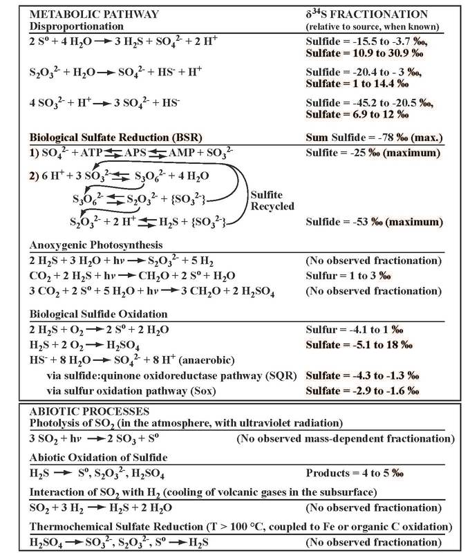
Table 1 (above) from the review paper tabulating biotic metabolic pathways involved with the sulfur cycle as well as abiotic processes, along with the known sulfur isotope fractionations associated.
|
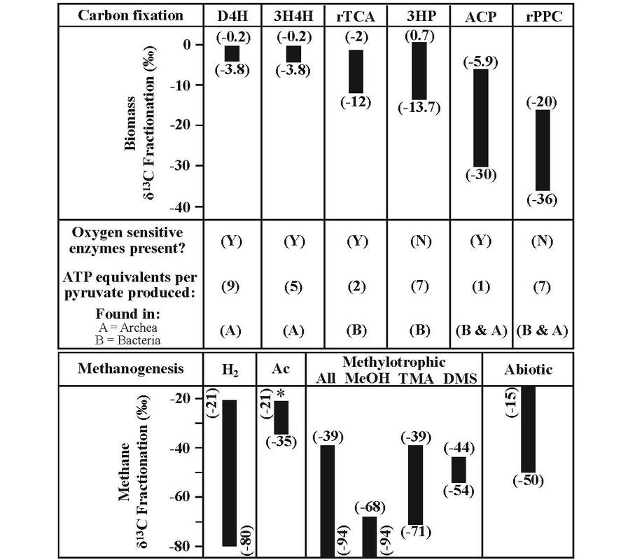
Table 2 (above) from the review paper tabulating carbon isotope fractionations associated with known carbon fixation pathways, the sensitivity and prevalence of those fixation pathways, and the fractionation associated with biotic and abiotic methanogenesis. Based on it's sensitivity to oxygen, extreme efficiency in ATP equivalents needed, and ubiquity, the Acetyl Co-enzyme A pathway (ACP) is the most likely candidate for the earliest carbon fixation pathway to evolve.
|

Figure 8 (left) from our review paper predicting the onset of sulfur-related metabolisms. The black bars represent our predictions based on S and C isotope data, and the white bars and points represent molecular clock calculations from the literature. It is important to note that these are for the modern pathways, and that messy/inefficient early versions of these pathways may have evolved earlier. As an example, while the modern Nitrogenase gene is thought to have evolved as early as 2.2 Ga, it is likely that a less efficient early version of the gene may have evolved earlier but was not preserved due to modern Nitrogenase being more robust and efficient, and thus out competing earlier versions which were relinquished to the molecular dust bin.
|
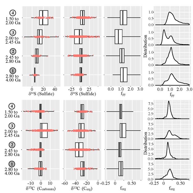
Figure 7 (above) shows sulfur (top) and carbon (bottom) isotopic composition and calculated fraction of burial (fpy and forg) done by Dr. Aviv Bachan. Data binned according to time periods described in the text. Each bin was randomly subsampled 1000 times and fpy or forg calculated on the pairs of points (shown in red) drawn from the reduced and oxidized species. The resulting calculated distribution for fpy and forg is plotted in the right two columns, once as a box plot and once as a kernel density plot.
|
MEDICINE BOW MOUNTAINS, WY (2.7 to 1.8 Ga)
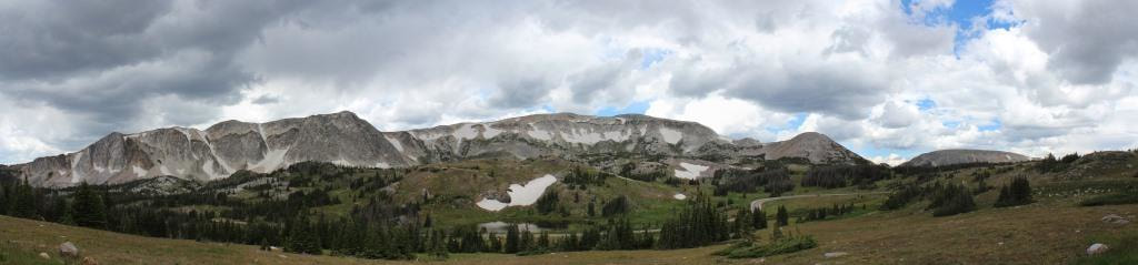
The Wyoming Craton has been dated to ~3.5 to 4.0 billion years old, and is one of several cratons that assembled into what is thought to have been the first continent on earth around 3.0 billion years ago. The Medicine Bow Mountains are a place where sedimentary rocks that were deposited on this first continent have been exposed thanks to tectonic forces pulling and pushing the continents as they move due to mantle currents. Some of these sediments were deposited during one of the most tumultuous times in earth history, when the surface of the earth transitioned from anoxic (reducing, with the atmosphere devoid of free oxygen), to having free oxygen in concentrations that may have been as much as 10 % of present day levels (depending on who you talk to, as there are different hypotheses and still much to learn).
The Nash Formation is a ~2.0 Ga carbonate unit that contains abundant evidence of microbial communities, including stromatolites. Some of the most positive carbon isotope values ever published (with carbonate δ13C values of almost +30 ‰) have come from this unit. The Nash Formation records a time when the geochemistry of the earth's surface abruptly transitioned from wildly fluctuating to relative quiescence, settling into what has been dubbed the 'boring billion' (though I beg to differ with this misnomer). We sampled the Medicine Bow Mountains during the summer of 2014, and again in the summer of 2019. Stay tuned, as we are planning on submitting a manuscript in the fall of 2019 that will include the work of Professor Katja Meyer from Willamette University in applying modeling to understanding the geochemistry of the site.
The Nash Formation is a ~2.0 Ga carbonate unit that contains abundant evidence of microbial communities, including stromatolites. Some of the most positive carbon isotope values ever published (with carbonate δ13C values of almost +30 ‰) have come from this unit. The Nash Formation records a time when the geochemistry of the earth's surface abruptly transitioned from wildly fluctuating to relative quiescence, settling into what has been dubbed the 'boring billion' (though I beg to differ with this misnomer). We sampled the Medicine Bow Mountains during the summer of 2014, and again in the summer of 2019. Stay tuned, as we are planning on submitting a manuscript in the fall of 2019 that will include the work of Professor Katja Meyer from Willamette University in applying modeling to understanding the geochemistry of the site.
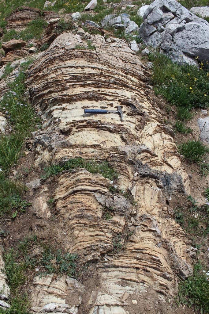
Large domal stromatolites outcrop in the middle of the Nash Formation. We were able to track this specific unit across a kilometer of transect. Photo by Jeff Havig.
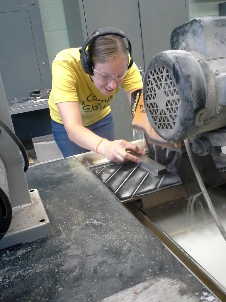
Anna Byers was instrumental in processing all of the samples collected from the 2014 expedition to the Medicine Bow Mountains. Here she is demonstrating excellent rock saw technique as she cuts a piece of shale. Photo by Jeff Havig.
|
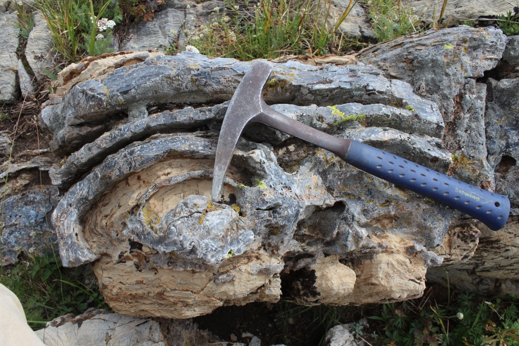
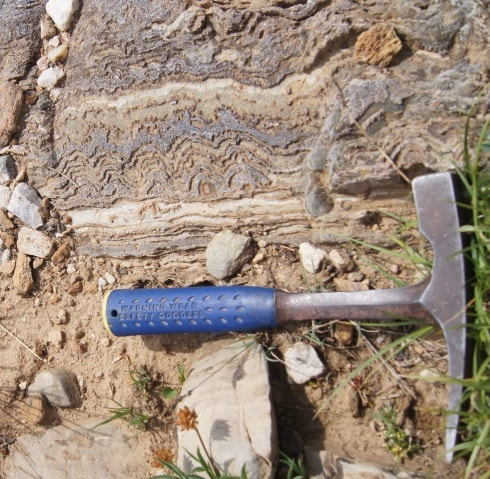
A stromatolite in the middle Nash Formation. Stromatolites are formed from microbial communities. The grey chert portion of the stromatolite is more resistant to weathering, while the tanish-brown dolomite (calcium-magnesium carbonate) is more susceptible, being slowly dissolved by carbonic acid formed when carbon dioxide in the atmosphere reacts with water. Photo by Jeff Havig.
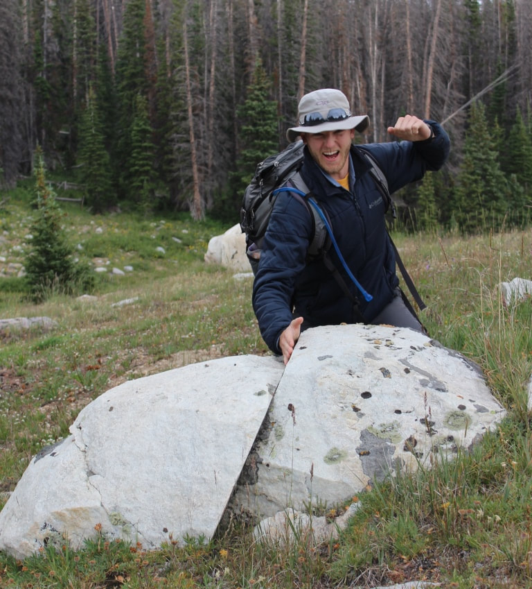
Dr. Kyle Rybacki is a force to be reckoned with in the field. Here he is demonstrating his first step in field thin section preparation on a hapless piece of Sugarloaf Quartzite. Photo by Jeff Havig.
|
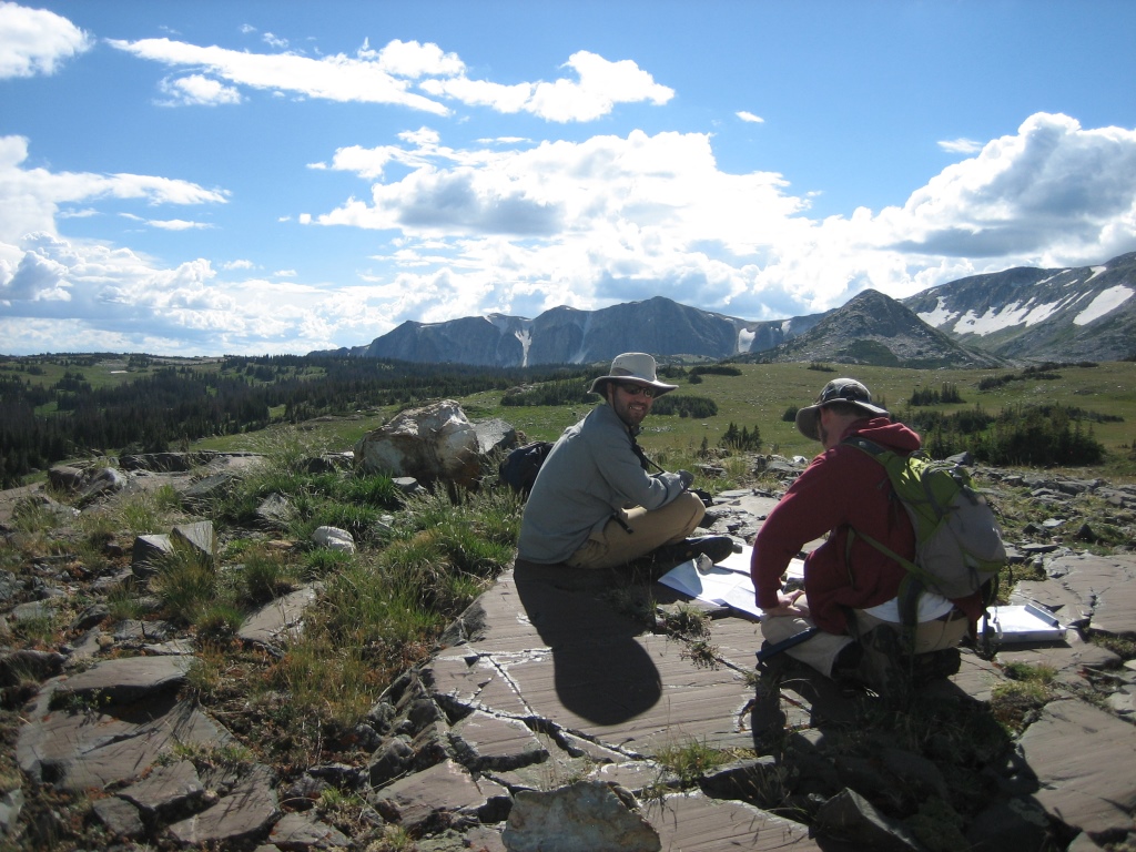
Dr. Aviv Bachan (left) and I 'discussing' our position on our topographic map while collecting samples. We are sitting on a mafic igneous intrusion in the Nash Formation that has been ground smooth by the action of glaciers during the last ice age. Photo by Kyle Rybacki.
The Towner Greenstone consisted of beautifully preserved pillow basalt flows immediately capping the Nash Formation carbonates. Photo by Jeff Havig.
Beautiful small-scale stromatolites and microbialites exposed in the Nash Fm. Photo by Jeff Havig.
|
The Colberg Metavolcanics are an approximately 2.7 Ga package of rocks that range from (predominantly) mafic to intermediate to felsic in composition, located in the northern portion of the Medicine Bow National Forest in the Medicine Bow Mountains. Regional mapping of the area in the late 1980s to early 1990s provided a great baseline for exploring the volcanic rocks. We explored the Colberg Metavolcanics in the summer of 2019.
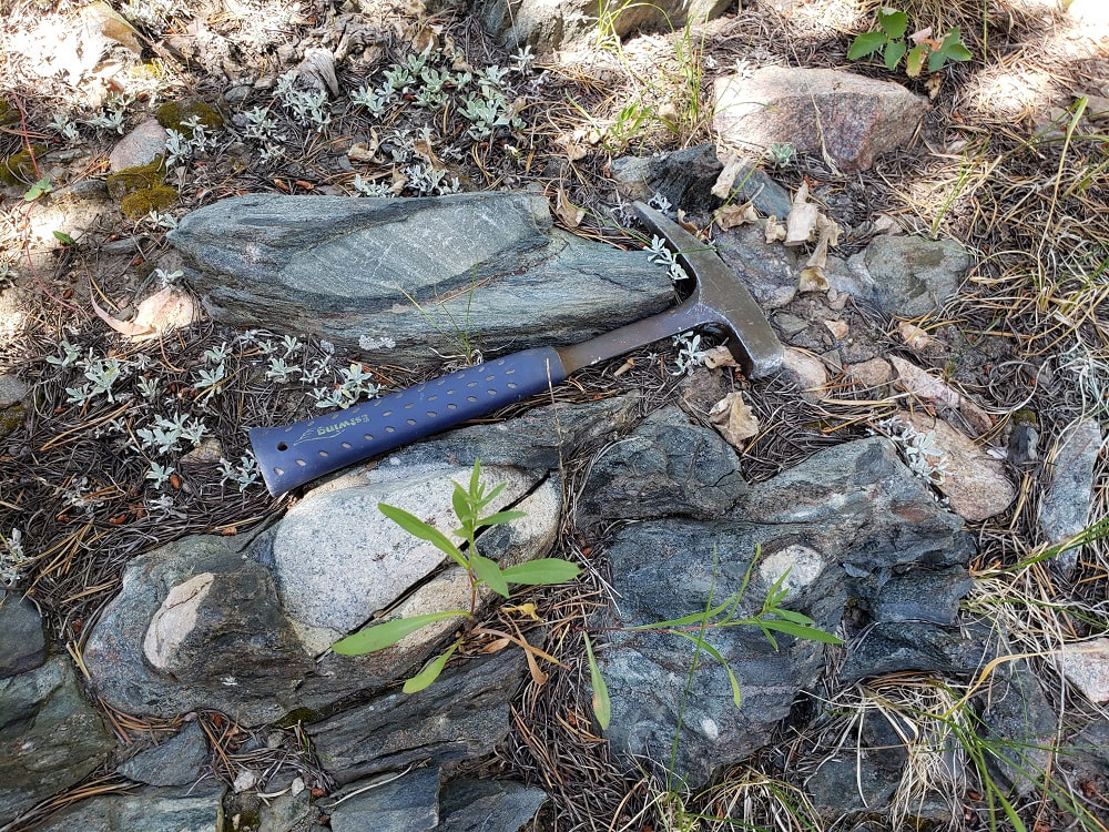
Above: Amygdaloidal Basalt in the Colberg Metavolcanics, suggesting the flow was subaerial (the amygdals being gas vesicles that were later filled in with minerals). Photo by Jeff Havig.
|
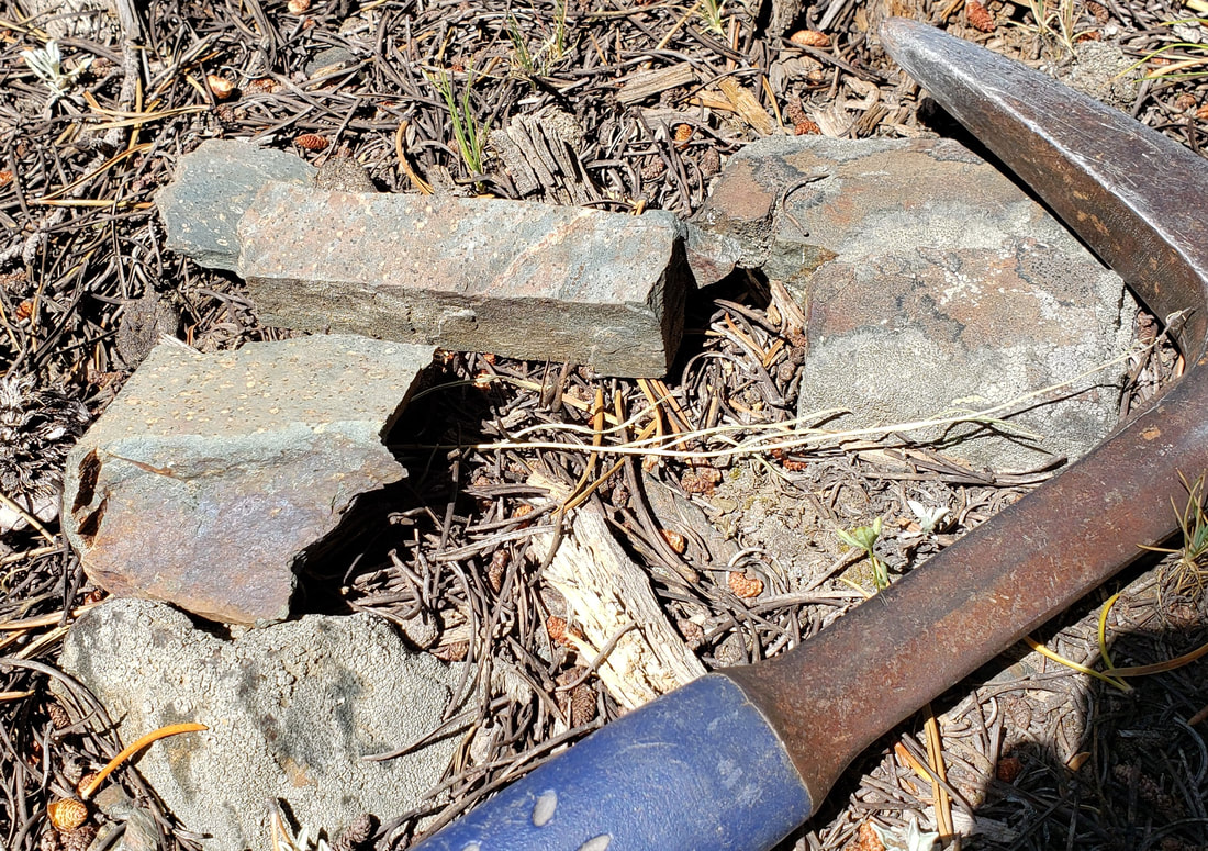
Below: Though hard to make out due to the lighting, I am holding what looks like a flow breccia, which forms at the flow fronts of lavas (in this case a basaltic lava). Photo by Jeff Havig.
|
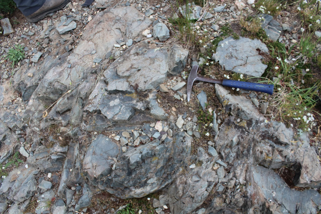
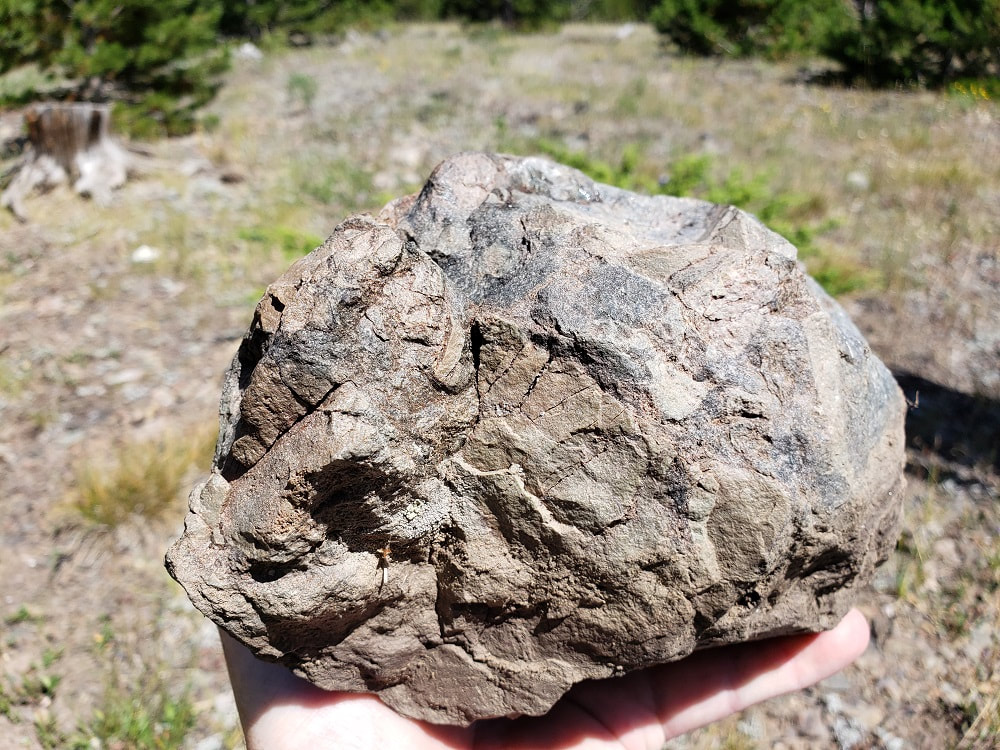
Above: A matrix supported conglomerate including rounded to sub-angular cobbles of granite (TTG), quartzite (sandstone), and mafic rocks. This reminded me of ash-dominant lahar deposits that often form in river channels of active volcanic regions. Photo by Jeff Havig.
|
DRESSER FORMATION, PILBARA, AUSTRALIA (3.48 Ga)
|
We are extremely fortunate in getting to collaborate with Professor Martin Van Kranendonk and PhD candidate Tara Djokic from the University of New South Wales in working to make connections between the modern hydrothermal features in Yellowstone National Park and their field site.
Tara is the first person to find evidence for subaerial hot spring deposits (including putative geyserite) in the Dresser Formation, which is a 3.48 billion year old volcanic setting including a caldera similar to that of Yellowstone. |
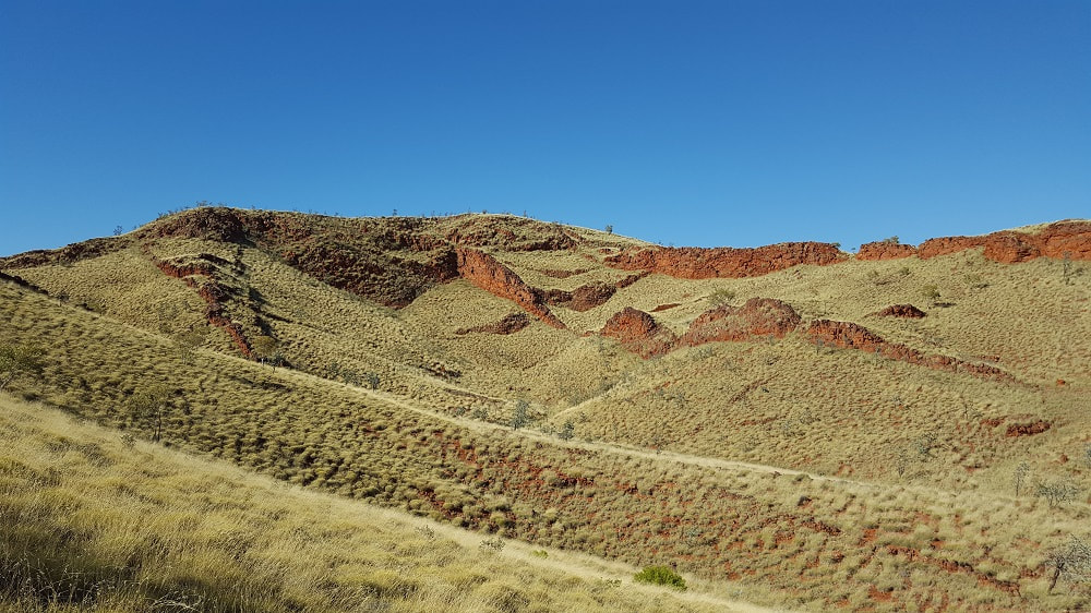
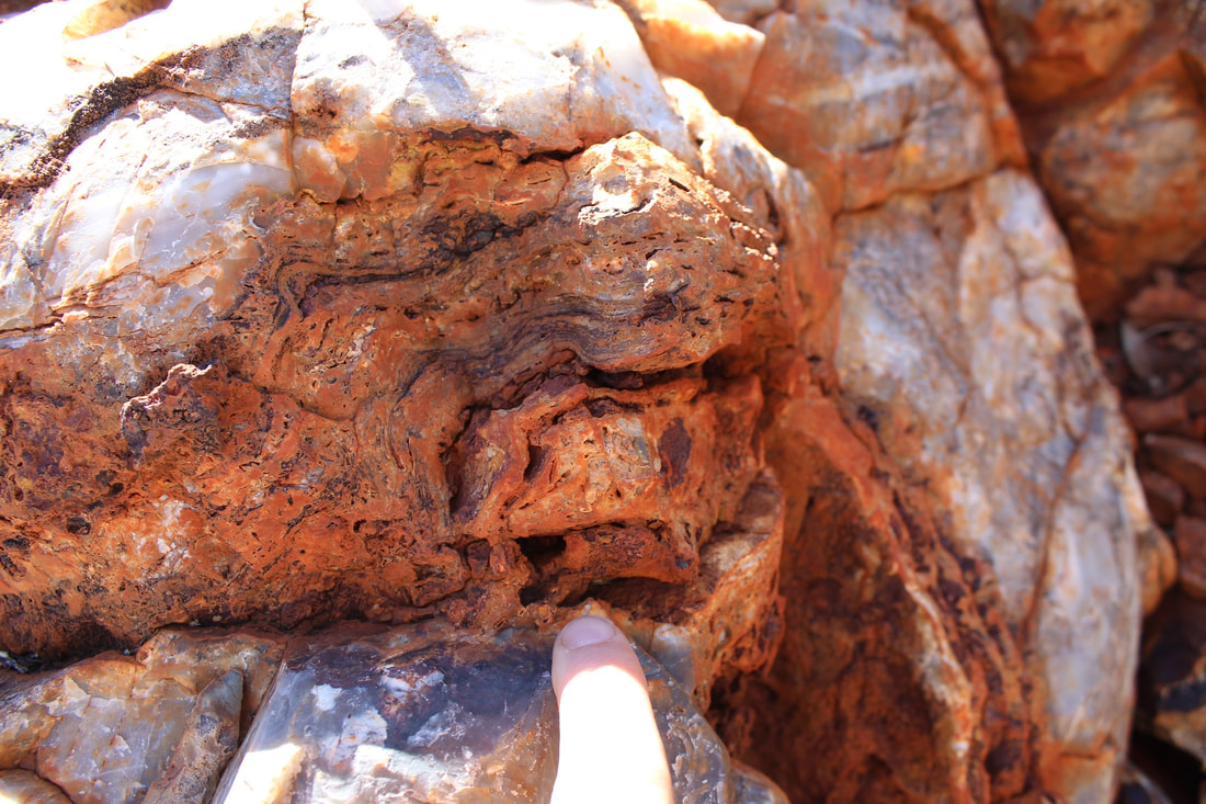
Above: The Dresser Formation has been tilted approximately 60 degrees away from the front of this image, exposing the underbelly of the hydrothermal system that was active at 3.48 Ga. The large wall-like features are quartz and barite containing veins highlighting the original underground plumbing that was feeding the putative hot springs. Photo by Jeff Havig.
Below: Tara's first publication on her work describing the putative hot spring deposits in the Dresser Formation.
|
Below: (Then PhD candidate) Dr. Tara Djokic giving a description of her research site. Note just how badass Tara is, as she is not wearing long pants OR gators in spite of the brutal and abundant spinifex grass all around her. Photo by Jeff Havig.

| ||||||
In a follow-up to Dr. Djokic's 2017 paper (above) first introducing the world to the terrestrial hot spring deposit that she discovered and described, her 2021 paper (below) is a tour de force with all the detail and exciting texture pictures that one could hope for. I count myself as being incredibly lucky in getting to host Tara as part of our 2018 Yellowstone sampling expedition team, giving us the opportunity to introduce her to all of the features that we work at. This collaborative effort resulted in my (very fortunate and appreciated) inclusion as a coauthor in the 2021 paper where many Yellowstone features are used as modern analogs for the textures described in the Dresser Fm. terrestrial hot spring outcrop. This collaboration is continuing with ongoing research by PhD candidate Michaela Dobson (University of Auckland), who is working on drill cores collected at the Dresser hot spring site in 2019. So stay tuned for more!
|
Below: Overview geologic map of the Dresser Fm. showing the context for the terrestrial hot spring outcrop. (Djokic et al., 2021)
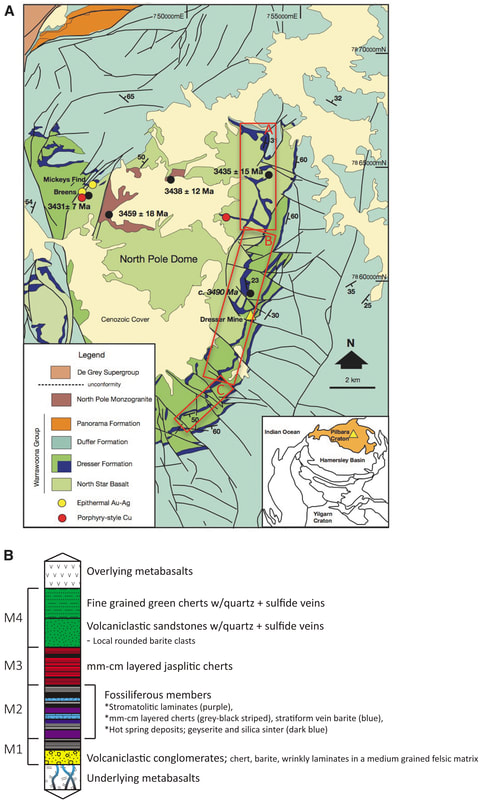
From Djokic et al. (2021): FIG. 1. (A) Geological map of the Dresser Formation in the North Pole Dome (modified from Harris et al., 2009). The lower chert-barite sequence (DFc1) of the Dresser Formation is the blue chert horizon highlighted by inset red boxes A, B, and C. Inset boxes also correspond to detailed geological maps: Supplementary Fig. S1A–C. (B) Generalized stratigraphy of DFc1.
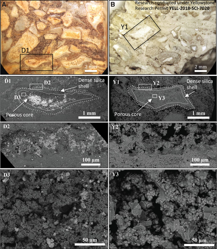
Above - A direct comparison of textures found in the Dresser Fm. with those we have found in Yellowstone. I was blown away with how the textures are identical, and how well those textures were preserved in a 3.5 billion year old rock!
From Djokic et al., 2021: FIG. 24. (A) Hand sample image of Dresser Formation breccia unit (Fig. 9): hash, showing inset box indicating SEM image of single angular fragment (D1)—Dashed line represents outer edge (D2). Inner dotted line indicates transition between porous core (D3) composed of Fe-oxide (light gray)+barite (white) and the dense, fine-grained rim of silica (dark gray). (B) Hand sample image of sinter breccia from an extinct hot spring in Norris Geyser Basin, YNP, USA, showing inset box indicating SEM image of sinter breccia (Y1)—Outer dashed line represents outer edge of sinter fragment (Y2). Inner dotted line indicates transition between microbially derived porous sinter core now containing silica spheres (Y3) and the dense coating of silica. SEM, scanning electron microscopy. |
Below: Tara's follow up publication in a special issue of the journal Astrobiology giving detailed descriptions and images of textures of the Dresser Fm. terrestrial hot spring deposits.
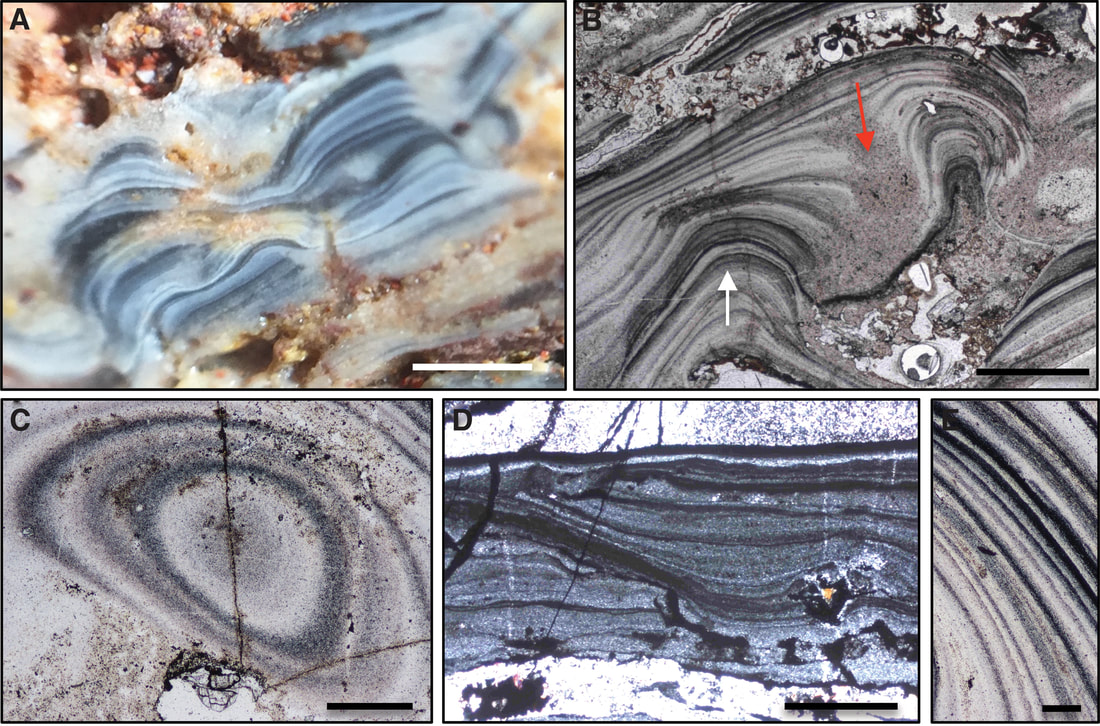
Above - Geyserite textures viewed in thin sections from the Dresser Fm. site.
From Djokic et al., 2021: FIG. 3. Dresser Formation geyserite. Scale bar measurements and polarized light indicated. (A) Botryoidal features in hand sample (2 mm). (B) Botryoids (white arrow) separated by equigranular troughs (red arrow) (1 mm, ppl). (C) Plan view of botryoid (1 mm, ppl). (D) Slump structures (1 mm, xpl). (E) Distinct fine scale black and white laminations characteristic of geyserite (100 μm, xpl). ppl, plane polarized light; xpl, crossed polarized light. Above - Geyserite textures viewed in thin sections from the Dresser Fm. site.
From Djokic et al., 2021: FIG. 3. Dresser Formation geyserite. Scale bar measurements and polarized light indicated. (A) Botryoidal features in hand sample (2 mm). (B) Botryoids (white arrow) separated by equigranular troughs (red arrow) (1 mm, ppl). (C) Plan view of botryoid (1 mm, ppl). (D) Slump structures (1 mm, xpl). (E) Distinct fine scale black and white laminations characteristic of geyserite (100 μm, xpl). ppl, plane polarized light; xpl, crossed polarized light. 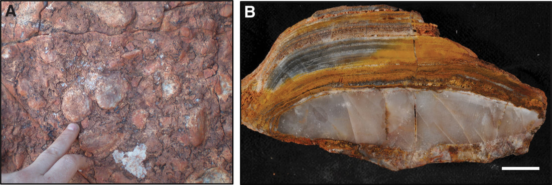
Above - A hand sample cross cut of textures we find in Yellowstone where microbial communities grow on pieces of sinter in pools and outflow channels.
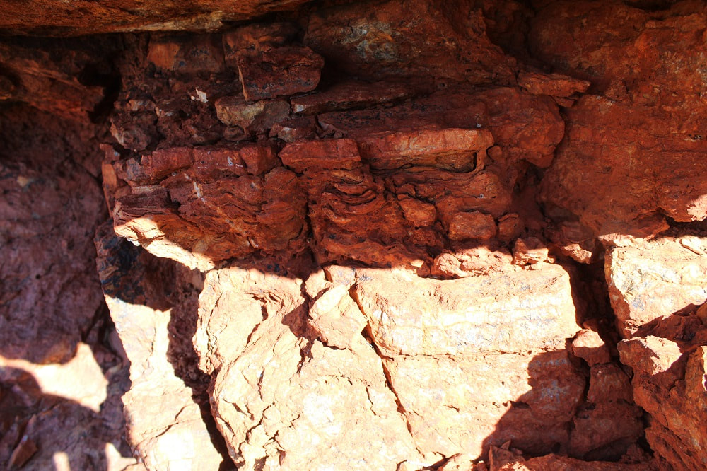
From Djokic et al., 2021: FIG. 8. Rounded pebble-to-cobble conglomerate in the Dresser Formation. Scale bar measurement indicated. (A) Outcrop image. (B) Cross-section showing white translucent chert pebble overlain by tourmaline-bearing wrinkly laminates (1 cm). Compare with Guido and Campbell (2019), their Figs. 2D and 3. 
Above - From Djokic et al., 2021: FIG. 22. Proximal vent facies—ancient and modern comparisons. Scale bar measurements and polarized light indicated. (A) Dresser geyserite cornices (100 μm, ppl) compared with (B) geyserite cornice from NZ sinter (250 μm, ppl). (C) Botryoidal geyserite with orange microbial mats growing in low-temperature niches at the base of a cobble adjacent to Boulder Geyser Creek, Lower Geyser Basin, YNP, USA (2 cm). (D) Slump textures in Dresser stratiform geyserite (500 μm, ppl) compared with (E) slump structures associated with NZ stratiform geyserite (500 μm). (F) Petrographic image of slump structures in (E) (500 μm, xpl). (G) Hot spring geyser pool in Lower Geyser Basin, YNP, USA. Red arrow—splash zone; columnar geyserite forming. Yellow arrow—pooling water; stratiform geyserite forming (0.5 m).
| ||
